| “Wonderful Data Visualization” Edward Tufte Keynote talk to China Visualization and Visual Analytics Conference (ChinaVis) |
| “Wonderful Data Visualization” Edward Tufte Keynote talk to China Visualization and Visual Analytics Conference (ChinaVis) |
by Edward Tufte |
|
E.T. |
Aug 4, 2022 |
| Edward Tufte presentation method caused Jeff Bezos, Amazon, AWS to throw out PowerPoint |
| Edward Tufte presentation method caused Jeff Bezos, Amazon, AWS to throw out PowerPoint |
by Edward Tufte |
|
E.T. |
Apr 26, 2022 |
| Visual Display of Quantitative Information: First Sketches |
| Visual Display of Quantitative Information: First Sketches |
by Edward Tufte |
|
E.T. |
Nov 25, 2020 |
| If most medical research is false, then what about research-on-research? |
| If most medical research is false, then what about research-on-research? |
by Edward Tufte |
|
E.T. |
Jul 16, 2019 |
| Practical Advice for Medical Patients |
| Practical Advice for Medical Patients |
by Edward Tufte |
|
E.T., Science |
Jan 28, 2019 |
| Displaying estimates +/- error, confidence bounds |
| Displaying estimates +/- error, confidence bounds |
by Edward Tufte |
|
E.T. |
Mar 9, 2017 |
| The crisis in data analysis: most published studies are false |
| The crisis in data analysis: most published studies are false |
by Edward Tufte |
|
E.T. |
Nov 15, 2016 |
| Sparklines History by Tufte: 1324 to now |
| Sparklines History by Tufte: 1324 to now |
by Edward Tufte |
|
E.T. |
Sep 22, 2016 |
| Edward Tufte course review: “Best one-day course your company can send you to” |
| Edward Tufte course review: “Best one-day course your company can send you to” |
by Staff |
|
|
Aug 15, 2016 |
| Edward Tufte course review: “One visionary day” WIRED |
| Edward Tufte course review: “One visionary day” WIRED |
by staff |
|
|
Aug 10, 2016 |
| Edward Tufte course reviews: 27 reviews of Tufte one-day class |
| Edward Tufte course reviews: 27 reviews of Tufte one-day class |
by Tufte course reviews |
|
|
Aug 9, 2016 |
| Sentences off the Grid |
| Sentences off the Grid |
by Edward Tufte |
|
Art, E.T., Science |
May 17, 2016 |
| Maya Lin, Women’s Table at Yale University, and ET |
| Maya Lin, Women’s Table at Yale University, and ET |
by Edward Tufte |
|
E.T. |
Mar 9, 2016 |
| Are diagrams the metaphor for Cubism? |
| Are diagrams the metaphor for Cubism? |
by Edward Tufte |
|
E.T. |
Mar 1, 2016 |
| First known statistical graphic |
| First known statistical graphic |
by Edward Tufte |
|
E.T. |
Feb 22, 2016 |
| Time-series that move through XY space |
| Time-series that move through XY space |
by Edward Tufte |
|
E.T. |
Feb 18, 2016 |
| Two- and Three-Dimensional Sentences |
| Two- and Three-Dimensional Sentences |
by Edward Tufte |
|
E.T. |
Feb 16, 2016 |
| Image Quilts |
| Image Quilts |
by Edward Tufte |
|
E.T. |
Sep 20, 2015 |
| Goldberg and Design Variations |
| Goldberg and Design Variations |
by Edward Tufte |
|
E.T., Science |
Aug 25, 2015 |
| Table and timetable design and typography |
| Table and timetable design and typography |
by Edward Tufte |
|
E.T., Science |
Aug 21, 2015 |
| Overlapping data graphics to make comparisons |
| Overlapping data graphics to make comparisons |
by Edward Tufte |
|
E.T., Science |
Jun 2, 2015 |
| Chartjunk |
| Chartjunk |
by Edward Tufte |
|
E.T., Science |
Jan 29, 2015 |
| Consulting stories |
| Consulting stories |
by Edward Tufte |
|
E.T. |
Nov 10, 2014 |
| Hogpen Hill Farms LLC: Architectural evergreens and ornamental grasses |
| Hogpen Hill Farms LLC: Architectural evergreens and ornamental grasses |
by Edward Tufte |
|
Art, E.T. |
Oct 30, 2014 |
| On the Edge, At the Margin: Contours, Surrounds, Frames |
| On the Edge, At the Margin: Contours, Surrounds, Frames |
by Edward Tufte |
|
E.T. |
Sep 13, 2014 |
| Graphical timetables |
| Graphical timetables |
by Edward Tufte |
|
E.T., Science |
Jun 10, 2014 |
| Boxplots data test |
| Boxplots data test |
by Edward Tufte |
|
E.T. |
Jan 16, 2014 |
| Design review: Improving a good news graphic |
| Design review: Improving a good news graphic |
by Edward Tufte |
|
E.T. |
Jan 14, 2014 |
| Design of walking maps, indoors and outdoors |
| Design of walking maps, indoors and outdoors |
by Edward Tufte |
|
Art, E.T., Science |
Nov 12, 2013 |
| Image data quilts: our new website |
| Image data quilts: our new website |
by Edward Tufte |
|
Art, E.T., Science |
Sep 11, 2013 |
| Making better inferences from statistical graphics Edward Tufte |
| Making better inferences from statistical graphics Edward Tufte |
by Edward Tufte |
|
E.T., Science |
Sep 1, 2013 |
| Stonespace and Airspace = Lacy Stone Walls |
| Stonespace and Airspace = Lacy Stone Walls |
by Edward Tufte |
|
Art, E.T. |
Aug 7, 2013 |
| Flowing Steel Confections |
| Flowing Steel Confections |
by Edward Tufte |
|
Art, E.T. |
Jul 20, 2013 |
| Maps moving in time: a standard of excellence for data displays |
| Maps moving in time: a standard of excellence for data displays |
by Edward Tufte |
|
E.T., Science |
Jun 11, 2013 |
| John Tukey, classic paper on statistical graphics |
| John Tukey, classic paper on statistical graphics |
by Edward Tufte |
|
E.T. |
Feb 21, 2013 |
| Hogpen Hill Farms artworks |
| Hogpen Hill Farms artworks |
by Edward Tufte |
|
Art, E.T. |
Feb 13, 2013 |
| Fitting simple multivariate models |
| Fitting simple multivariate models |
by Edward Tufte |
|
E.T., Science |
Jan 23, 2013 |
| Ironstone artworks, torqued steel |
| Ironstone artworks, torqued steel |
by Edward Tufte |
|
Art, E.T., Sculpture |
Jan 20, 2013 |
| Two-variable linear regression |
| Two-variable linear regression |
by Edward Tufte |
|
E.T., Science |
Jan 14, 2013 |
| Predictions and projections: some issues of research design |
| Predictions and projections: some issues of research design |
by Edward Tufte |
|
E.T., Science |
Jan 10, 2013 |
| The meaning of “pessimal” |
| The meaning of “pessimal” |
by Edward Tufte |
|
E.T., Science |
Jan 7, 2013 |
| Megaliths, Continuous and Silent, Stuctures of Unknown Significance |
| Megaliths, Continuous and Silent, Stuctures of Unknown Significance |
by Edward Tufte |
|
Art, E.T., Sculpture |
Jan 3, 2013 |
| Rocket Science 3: Airstream Interplanetary Explorer |
| Rocket Science 3: Airstream Interplanetary Explorer |
by Edward Tufte |
|
Art, E.T., Science, Sculpture |
Jan 2, 2013 |
| Fitting models to data |
| Fitting models to data |
by Edward Tufte |
|
E.T., Science |
Dec 26, 2012 |
| Taking logarithms in statistical data |
| Taking logarithms in statistical data |
by Edward Tufte |
|
E.T., Science |
Nov 28, 2012 |
| Open space creation |
| Open space creation |
by Edward Tufte |
|
E.T. |
Nov 1, 2012 |
| Jakob Nielsen’s review of amazon’s Fire |
| Jakob Nielsen’s review of amazon’s Fire |
by Edward Tufte |
|
E.T. |
Dec 13, 2011 |
| Touchscreens have no hand |
| Touchscreens have no hand |
by Edward Tufte |
|
E.T., Science |
Nov 9, 2011 |
| Ace and Porta do multimedia |
| Ace and Porta do multimedia |
by Edward Tufte |
|
Art, E.T., Sculpture |
Nov 1, 2011 |
| Shadows |
| Shadows |
by Edward Tufte |
|
E.T., Science |
Nov 1, 2011 |
| Sculptures in the October storm |
| Sculptures in the October storm |
by Edward Tufte |
|
E.T. |
Nov 1, 2011 |
| The US Patent and Trademark Office creates a really stupid interface |
| The US Patent and Trademark Office creates a really stupid interface |
by Edward Tufte |
|
E.T. |
Oct 14, 2011 |
| Philosophical Diamond Signs |
| Philosophical Diamond Signs |
by Edward Tufte |
|
Art, E.T., Sculpture |
Oct 13, 2011 |
| Masks Quartet, 2011 |
| Masks Quartet, 2011 |
by Edward Tufte |
|
Art, E.T., Sculpture |
Sep 27, 2011 |
| Feynman Diagrams, Edward Tufte sculptures and exhibits |
| Feynman Diagrams, Edward Tufte sculptures and exhibits |
by Edward Tufte |
|
Art, E.T., Science, Sculpture |
Aug 25, 2011 |
| Sparkline > Steve Jobs > Andy Warhol in Google results |
| Sparkline > Steve Jobs > Andy Warhol in Google results |
by Edward Tufte |
|
E.T., Science |
Jul 11, 2011 |
| Slopegraphs for comparing gradients: Slopegraph theory and practice |
| Slopegraphs for comparing gradients: Slopegraph theory and practice |
by Edward Tufte |
|
E.T., Science |
Jun 1, 2011 |
| ET Reviews Some Books |
| ET Reviews Some Books |
by Edward Tufte |
|
E.T. |
Apr 2, 2011 |
| Classic articles on statistical thinking |
| Classic articles on statistical thinking |
by Edward Tufte |
|
E.T. |
Apr 2, 2011 |
| The work of Charles Joseph Minard |
| The work of Charles Joseph Minard |
by Edward Tufte |
|
E.T. |
Apr 2, 2011 |
| Graphical summaries for medical patients |
| Graphical summaries for medical patients |
by Edward Tufte |
|
E.T. |
Apr 2, 2011 |
| Light painting, a brilliant technique |
| Light painting, a brilliant technique |
by Edward Tufte |
|
E.T. |
Mar 20, 2011 |
| About ET: Edward Tufte interviews, biography, contact information |
| About ET: Edward Tufte interviews, biography, contact information |
by Edward Tufte |
|
E.T. |
Mar 19, 2011 |
| Sculpture Forgings |
| Sculpture Forgings |
by Edward Tufte |
|
Art, E.T., Sculpture |
Mar 6, 2011 |
| Christie’s auction of ET rare books: what’s going on |
| Christie’s auction of ET rare books: what’s going on |
by Edward Tufte |
|
E.T. |
Nov 12, 2010 |
| Displays of movie-making techniques |
| Displays of movie-making techniques |
by Edward Tufte |
|
E.T. |
Jul 12, 2010 |
| ET Modern |
| ET Modern |
by Edward Tufte |
|
E.T., Sculpture |
Jun 3, 2010 |
| Statistics at the FDA |
| Statistics at the FDA |
by Edward Tufte |
|
E.T. |
Apr 15, 2010 |
| Microsoft’s Courier digital journal (Courier cancelled, April 29, 2010) |
| Microsoft’s Courier digital journal (Courier cancelled, April 29, 2010) |
by Edward Tufte |
|
E.T. |
Mar 7, 2010 |
| Windows Phone 7 Series (WP7S) |
| Windows Phone 7 Series (WP7S) |
by Edward Tufte |
|
E.T. |
Feb 17, 2010 |
| Data displays for self-awareness |
| Data displays for self-awareness |
by Edward Tufte |
|
E.T. |
Feb 10, 2010 |
| Solari train boards |
| Solari train boards |
by Edward Tufte |
|
E.T. |
Jan 3, 2010 |
| 12 Reviews, ET Art Exhibits |
| 12 Reviews, ET Art Exhibits |
by Edward Tufte |
|
Art, E.T., Featured, Sculpture |
Dec 21, 2009 |
| Edward Burtynsky: Oil |
| Edward Burtynsky: Oil |
by Edward Tufte |
|
E.T. |
Nov 25, 2009 |
| ET show at George Champion Modern Shop |
| ET show at George Champion Modern Shop |
by Edward Tufte |
|
E.T., Sculpture |
Nov 19, 2009 |
| Microsoft patent claim for “sparklines in the grid” |
| Microsoft patent claim for “sparklines in the grid” |
by Edward Tufte |
|
E.T. |
Nov 19, 2009 |
| Whitney Museum: website redesign |
| Whitney Museum: website redesign |
by Edward Tufte |
|
E.T. |
Nov 13, 2009 |
| T. S. Eliot connection |
| T. S. Eliot connection |
by Dennis Kear |
|
|
Nov 5, 2009 |
| Claude Lévi-Strauss on pseudo-theory |
| Claude Lévi-Strauss on pseudo-theory |
by Edward Tufte |
|
E.T. |
Nov 4, 2009 |
| Rocket Science #2 (Lunar Lander) |
| Rocket Science #2 (Lunar Lander) |
by Edward Tufte |
|
Art, E.T., Sculpture |
Jun 2, 2009 |
| Microsoft’s CEO wants ET method of presentation, not PowerPoint |
| Microsoft’s CEO wants ET method of presentation, not PowerPoint |
by Edward Tufte |
|
E.T., Science |
May 18, 2009 |
| Magritte’s Smile |
| Magritte’s Smile |
by Edward Tufte |
|
Art, E.T., Sculpture |
May 12, 2009 |
| Telestrator–the electronic crayon |
| Telestrator–the electronic crayon |
by Edward Tufte |
|
E.T. |
Apr 23, 2009 |
| The Drawing Center fax show: ET exhibits |
| The Drawing Center fax show: ET exhibits |
by Edward Tufte |
|
Art, E.T., Sculpture |
Apr 15, 2009 |
| Describing and tracking stimulus projects totaling $787,000,000,000 on the internet: any ideas? |
| Describing and tracking stimulus projects totaling $787,000,000,000 on the internet: any ideas? |
by Edward Tufte |
|
E.T. |
Apr 12, 2009 |
| Digital books (and how to put ET books on the iPad) |
| Digital books (and how to put ET books on the iPad) |
by Edward Tufte |
|
E.T. |
Mar 27, 2009 |
| Abstract alley art |
| Abstract alley art |
by Edward Tufte |
|
Art, E.T. |
Mar 25, 2009 |
| Excel’s statistical graphics |
| Excel’s statistical graphics |
by Edward Tufte |
|
E.T. |
Mar 21, 2009 |
| Designing a museum sculpture garden: land, trees, artworks |
| Designing a museum sculpture garden: land, trees, artworks |
by Edward Tufte |
|
Art, E.T. |
Mar 9, 2009 |
| Outdoor benches |
| Outdoor benches |
by Edward Tufte |
|
E.T. |
Mar 9, 2009 |
| Financial data displays |
| Financial data displays |
by Edward Tufte |
|
E.T. |
Mar 4, 2009 |
| ET work on iTunes (Podcast), YouTube, Vimeo |
| ET work on iTunes (Podcast), YouTube, Vimeo |
by Edward Tufte |
|
E.T. |
Dec 31, 2008 |
| Slide show pan/zoom for museum computer screens: advice needed |
| Slide show pan/zoom for museum computer screens: advice needed |
by Edward Tufte |
|
E.T. |
Dec 30, 2008 |
| Data mining coincidences: Bellwether electoral districts |
| Data mining coincidences: Bellwether electoral districts |
by Edward Tufte |
|
E.T. |
Dec 3, 2008 |
| Rainbows and Moonbows |
| Rainbows and Moonbows |
by Edward Tufte |
|
E.T. |
Dec 1, 2008 |
| Airspaces |
| Airspaces |
by Edward Tufte |
|
Art, E.T., Sculpture |
Nov 20, 2008 |
| Election data displays |
| Election data displays |
by Edward Tufte |
|
E.T. |
Nov 4, 2008 |
| Dog sculpture (Porta the Portuguese Water Dog) |
| Dog sculpture (Porta the Portuguese Water Dog) |
by Edward Tufte |
|
Art, E.T., Sculpture |
Oct 29, 2008 |
| Distant assistants: real-time collaboration |
| Distant assistants: real-time collaboration |
by Edward Tufte |
|
E.T. |
Oct 16, 2008 |
| Cartoon maps of ET books |
| Cartoon maps of ET books |
by Edward Tufte |
|
E.T. |
Oct 9, 2008 |
| Scaling and scale models |
| Scaling and scale models |
by Edward Tufte |
|
E.T., Science |
Sep 8, 2008 |
| Google Chrome platform |
| Google Chrome platform |
by Tchad |
|
|
Sep 3, 2008 |
| BibliOdyssey: wonderful website about illustrations |
| BibliOdyssey: wonderful website about illustrations |
by Edward Tufte |
|
E.T. |
Aug 23, 2008 |
| Seeing Around: New ET essay published |
| Seeing Around: New ET essay published |
by Edward Tufte |
|
Art, E.T., Sculpture |
Aug 12, 2008 |
| Paradox sculptures |
| Paradox sculptures |
by Edward Tufte |
|
E.T., Sculpture |
Aug 12, 2008 |
| Theater Museum artworks |
| Theater Museum artworks |
by Edward Tufte |
|
E.T., Sculpture |
Aug 11, 2008 |
| Calendars and schedules |
| Calendars and schedules |
by Simon Shutter |
|
|
Jun 16, 2008 |
| Geese taking flight (at 300 frames per second) |
| Geese taking flight (at 300 frames per second) |
by Edward Tufte |
|
Art, E.T., Science |
Jun 9, 2008 |
| Gentle humor in design |
| Gentle humor in design |
by Edward Tufte |
|
E.T. |
Jun 3, 2008 |
| Complex sculptural shapes |
| Complex sculptural shapes |
by Edward Tufte |
|
E.T., Sculpture |
Jun 2, 2008 |
| Porta and the Birds (at 300 frames/second) |
| Porta and the Birds (at 300 frames/second) |
by Edward Tufte |
|
Art, E.T. |
Jun 2, 2008 |
| See now . . . Words later |
| See now . . . Words later |
by Edward Tufte |
|
E.T. |
May 19, 2008 |
| Early ET works: paintings, constructions |
| Early ET works: paintings, constructions |
by Edward Tufte |
|
E.T. |
Apr 21, 2008 |
| Resolution and dimensional compression |
| Resolution and dimensional compression |
by Edward Tufte |
|
E.T. |
Apr 17, 2008 |
| Flame Theater |
| Flame Theater |
by Edward Tufte |
|
Art, E.T., Sculpture |
Apr 6, 2008 |
| 714,032 pageviews by Microsoft IP number to our shopping cart in 3 days: what’s going on? |
| 714,032 pageviews by Microsoft IP number to our shopping cart in 3 days: what’s going on? |
by Edward Tufte |
|
E.T. |
Mar 15, 2008 |
| Tong Bird of Paradise |
| Tong Bird of Paradise |
by Edward Tufte |
|
Art, E.T., Sculpture |
Feb 18, 2008 |
| Olafur Eliasson: Take Your Time |
| Olafur Eliasson: Take Your Time |
by Edward Tufte |
|
E.T. |
Feb 13, 2008 |
| Open-Ended |
| Open-Ended |
by Edward Tufte |
|
E.T., Sculpture |
Feb 11, 2008 |
| Elegant water drainage methods: Levi Plaza in San Francisco and elsewhere |
| Elegant water drainage methods: Levi Plaza in San Francisco and elsewhere |
by Edward Tufte |
|
E.T. |
Feb 6, 2008 |
| Residing in spaceland: Johnny Chung Lee’s imaginative work |
| Residing in spaceland: Johnny Chung Lee’s imaginative work |
by Edward Tufte |
|
E.T. |
Feb 3, 2008 |
| iPhone interface design |
| iPhone interface design |
by Edward Tufte |
|
E.T., Science |
Jan 21, 2008 |
| Georgia O’Keeffe and Escaping Flatland |
| Georgia O’Keeffe and Escaping Flatland |
by Edward Tufte |
|
E.T., Sculpture |
Jan 9, 2008 |
| Maintaining at least some privacy on the internet |
| Maintaining at least some privacy on the internet |
by Edward Tufte |
|
E.T. |
Dec 27, 2007 |
| ZZ Smile (Zerlina’s Smile) |
| ZZ Smile (Zerlina’s Smile) |
by Edward Tufte |
|
Art, E.T., Sculpture |
Dec 20, 2007 |
| Rocket Science |
| Rocket Science |
by Edward Tufte |
|
Art, E.T., Sculpture |
Nov 15, 2007 |
| Buddha with Bird Nest: sculpture |
| Buddha with Bird Nest: sculpture |
by Edward Tufte |
|
Art, E.T., Sculpture |
Nov 7, 2007 |
| Major show of ET artwork at The Aldrich Contemporary Art Museum |
| Major show of ET artwork at The Aldrich Contemporary Art Museum |
by Edward Tufte |
|
E.T. |
Oct 2, 2007 |
| Sheep visit landscape sculpture |
| Sheep visit landscape sculpture |
by Edward Tufte |
|
Art, E.T. |
Oct 2, 2007 |
| Skewed Machine |
| Skewed Machine |
by Edward Tufte |
|
Art, E.T., Sculpture |
Aug 21, 2007 |
| Unusual maps |
| Unusual maps |
by Edward Tufte |
|
E.T. |
Aug 7, 2007 |
| Megan Jaegerman’s brilliant news graphics |
| Megan Jaegerman’s brilliant news graphics |
by Edward Tufte |
|
E.T., Science |
Jun 28, 2007 |
| Notebooks for Project 5 |
| Notebooks for Project 5 |
by Edward Tufte |
|
E.T. |
Jun 21, 2007 |
| Wavefields: intense animated data graphics |
| Wavefields: intense animated data graphics |
by Edward Tufte |
|
E.T., Science |
Jun 21, 2007 |
| Multiplicity in visual experiences (ET presentation for a museum show) |
| Multiplicity in visual experiences (ET presentation for a museum show) |
by Edward Tufte |
|
E.T., Sculpture |
Jun 11, 2007 |
| Water studies: light and motion |
| Water studies: light and motion |
by Edward Tufte |
|
E.T. |
May 29, 2007 |
| Documentation sketches |
| Documentation sketches |
by Edward Tufte |
|
E.T. |
May 17, 2007 |
| Steel sculptures |
| Steel sculptures |
by Edward Tufte |
|
E.T., Sculpture |
Apr 12, 2007 |
| Dappled light |
| Dappled light |
by Edward Tufte |
|
E.T., Science |
Apr 10, 2007 |
| Sculpture: Negative space studies |
| Sculpture: Negative space studies |
by Edward Tufte |
|
E.T., Sculpture |
Apr 6, 2007 |
| David Hockney: Secret Knowledge |
| David Hockney: Secret Knowledge |
by Edward Tufte |
|
E.T. |
Mar 29, 2007 |
| Experimental two-day course on July 12-13 in Palo Alto, California |
| Experimental two-day course on July 12-13 in Palo Alto, California |
by Edward Tufte |
|
E.T. |
Mar 27, 2007 |
| Pine needles in the snow: physical and optical effects |
| Pine needles in the snow: physical and optical effects |
by Edward Tufte |
|
E.T. |
Mar 23, 2007 |
| About ET: Esquire, New York Magazine, Stanford Magazine |
| About ET: Esquire, New York Magazine, Stanford Magazine |
by Edward Tufte |
|
E.T. |
Mar 22, 2007 |
| ET Primitive Art |
| ET Primitive Art |
by Edward Tufte |
|
E.T. |
Mar 20, 2007 |
| Survival vs. mortality results from cancer detection |
| Survival vs. mortality results from cancer detection |
by Edward Tufte |
|
E.T. |
Mar 13, 2007 |
| Cleaning up Excel’s poshlust graphics |
| Cleaning up Excel’s poshlust graphics |
by Edward Tufte |
|
E.T. |
Mar 8, 2007 |
| Table sculptures |
| Table sculptures |
by Edward Tufte |
|
Art, E.T., Sculpture |
Mar 8, 2007 |
| ET talk at Harvard, February 21, 2007 |
| ET talk at Harvard, February 21, 2007 |
by Edward Tufte |
|
E.T. |
Feb 16, 2007 |
| Richard Feynman’s “Nature cannot be fooled” |
| Richard Feynman’s “Nature cannot be fooled” |
by Edward Tufte |
|
E.T., Science |
Feb 5, 2007 |
| Ryszard Kapuscinski |
| Ryszard Kapuscinski |
by Edward Tufte |
|
E.T. |
Jan 25, 2007 |
| Stainless steel images: anisotropic calligraphy |
| Stainless steel images: anisotropic calligraphy |
by Edward Tufte |
|
Art, E.T., Sculpture |
Jan 22, 2007 |
| Punctuation typography |
| Punctuation typography |
by Edward Tufte |
|
E.T. |
Jan 21, 2007 |
| Images as logos |
| Images as logos |
by Edward Tufte |
|
E.T. |
Jan 11, 2007 |
| Showing 3D measurement scales in 2D images (including astronomical pictures) |
| Showing 3D measurement scales in 2D images (including astronomical pictures) |
by Edward Tufte |
|
E.T. |
Dec 28, 2006 |
| Multiple exposure experiments |
| Multiple exposure experiments |
by Edward Tufte |
|
E.T. |
Dec 26, 2006 |
| Bouquet sculpture series–and Walking, Seeing, Constructing |
| Bouquet sculpture series–and Walking, Seeing, Constructing |
by Edward Tufte |
|
Art, E.T., Sculpture |
Dec 21, 2006 |
| Advice for effective analytical reasoning |
| Advice for effective analytical reasoning |
by Edward Tufte |
|
E.T., Science |
Dec 17, 2006 |
| Evidence blocking: secrets, censorship, and cover-ups as threats to learning the truth |
| Evidence blocking: secrets, censorship, and cover-ups as threats to learning the truth |
by Edward Tufte |
|
E.T. |
Nov 30, 2006 |
| Intolerance of free speech at colleges |
| Intolerance of free speech at colleges |
by Edward Tufte |
|
E.T. |
Nov 12, 2006 |
| Grand truths about human behavior |
| Grand truths about human behavior |
by Edward Tufte |
|
E.T., Science |
Nov 10, 2006 |
| Plagiarism detection in PowerPoint presentations |
| Plagiarism detection in PowerPoint presentations |
by Edward Tufte |
|
E.T., Science |
Oct 24, 2006 |
| YouTube as an arts performance encyclopedia |
| YouTube as an arts performance encyclopedia |
by Edward Tufte |
|
E.T. |
Oct 16, 2006 |
| Scientific visualization: evidence and/or fireworks |
| Scientific visualization: evidence and/or fireworks |
by Edward Tufte |
|
E.T. |
Sep 28, 2006 |
| Art Theorists Speak Out Cartoonishly |
| Art Theorists Speak Out Cartoonishly |
by Edward Tufte |
|
Art, E.T. |
Sep 27, 2006 |
| Forecasting oil resources |
| Forecasting oil resources |
by Edward Tufte |
|
E.T. |
Sep 25, 2006 |
| “Public art” |
| “Public art” |
by Edward Tufte |
|
E.T. |
Sep 11, 2006 |
| Metaphors, analogies, thought mappings |
| Metaphors, analogies, thought mappings |
by Edward Tufte |
|
E.T. |
Sep 10, 2006 |
| Evidence presentations: At the leading edge of serious practice |
| Evidence presentations: At the leading edge of serious practice |
by Edward Tufte |
|
E.T. |
Sep 6, 2006 |
| Organized stones in nature and architecture (puzzle stones) |
| Organized stones in nature and architecture (puzzle stones) |
by Edward Tufte |
|
E.T. |
Aug 31, 2006 |
| Measuring website traffic |
| Measuring website traffic |
by Edward Tufte |
|
E.T. |
Aug 29, 2006 |
| Lists: design and construction, by Edward Tufte |
| Lists: design and construction, by Edward Tufte |
by Edward Tufte |
|
E.T., Science |
Aug 28, 2006 |
| Hogpen Hill #1: sculpture installed August 2006 |
| Hogpen Hill #1: sculpture installed August 2006 |
by Edward Tufte |
|
Art, E.T., Sculpture |
Aug 28, 2006 |
| Lousy PowerPoint presentations: The fault of PP users? |
| Lousy PowerPoint presentations: The fault of PP users? |
by Edward Tufte |
|
E.T., Science |
Aug 21, 2006 |
| The Vitality of Mythical Numbers |
| The Vitality of Mythical Numbers |
by Edward Tufte |
|
E.T. |
Aug 16, 2006 |
| Escaping Flatland sculptures |
| Escaping Flatland sculptures |
by Edward Tufte |
|
E.T., Sculpture |
Aug 16, 2006 |
| Bird Books |
| Bird Books |
by Edward Tufte |
|
E.T. |
Aug 8, 2006 |
| The print clock: a method for dating early books and prints |
| The print clock: a method for dating early books and prints |
by Edward Tufte |
|
E.T. |
Aug 1, 2006 |
| Airport maps and runway incursions |
| Airport maps and runway incursions |
by Edward Tufte |
|
E.T., Science |
Jul 31, 2006 |
| Retina communicates to brain at 10 million bits per second: Implications for evidence displays? |
| Retina communicates to brain at 10 million bits per second: Implications for evidence displays? |
by Edward Tufte |
|
E.T. |
Jul 26, 2006 |
| Popular Music: The Classic Graphic by Reebee Garofalo |
| Popular Music: The Classic Graphic by Reebee Garofalo |
by Edward Tufte |
|
E.T. |
Jul 25, 2006 |
| Music videos with information design material |
| Music videos with information design material |
by Edward Tufte |
|
E.T. |
Jul 16, 2006 |
| Petals 1-3 |
| Petals 1-3 |
by Edward Tufte |
|
E.T., Sculpture |
Jun 21, 2006 |
| Jean Tinguely: Water-machines sculpture, sprinklers gone wild |
| Jean Tinguely: Water-machines sculpture, sprinklers gone wild |
by Edward Tufte |
|
E.T. |
Jun 21, 2006 |
| A visit to John Snow’s cholera-infected waterpump in London |
| A visit to John Snow’s cholera-infected waterpump in London |
by Edward Tufte |
|
E.T. |
Jun 19, 2006 |
| Towers: a new memorial for 9/11 |
| Towers: a new memorial for 9/11 |
by Edward Tufte |
|
E.T., Sculpture |
Jun 8, 2006 |
| Dear Leader I: landscape sculpture May 2006 |
| Dear Leader I: landscape sculpture May 2006 |
by Edward Tufte |
|
Art, E.T., Sculpture |
Jun 1, 2006 |
| Excessively hierarchical organization of information |
| Excessively hierarchical organization of information |
by Edward Tufte |
|
E.T. |
May 21, 2006 |
| Midterm congressional elections: ET papers |
| Midterm congressional elections: ET papers |
by Edward Tufte |
|
E.T. |
May 9, 2006 |
| Horizons, vistas, and skylines |
| Horizons, vistas, and skylines |
by Edward Tufte |
|
Art, E.T. |
Mar 27, 2006 |
| Museum visits |
| Museum visits |
by Edward Tufte |
|
E.T. |
Mar 20, 2006 |
| How to discover asteroid impacts |
| How to discover asteroid impacts |
by Edward Tufte |
|
E.T. |
Mar 11, 2006 |
| Interfacing with voice mail menu systems vs. humans |
| Interfacing with voice mail menu systems vs. humans |
by Edward Tufte |
|
E.T. |
Feb 26, 2006 |
| Artful Sentences: Syntax as Style by Virginia Tufte now published! |
| Artful Sentences: Syntax as Style by Virginia Tufte now published! |
by Edward Tufte |
|
E.T. |
Feb 23, 2006 |
| Mass production of high-resolution digital prints–help needed |
| Mass production of high-resolution digital prints–help needed |
by Edward Tufte |
|
E.T. |
Feb 19, 2006 |
| Medicare prescription drug plan fiasco |
| Medicare prescription drug plan fiasco |
by Edward Tufte |
|
E.T. |
Feb 14, 2006 |
| Not everyone knows what quote marks mean in a search entry |
| Not everyone knows what quote marks mean in a search entry |
by Edward Tufte |
|
E.T. |
Feb 11, 2006 |
| Dan Flavin’s light works |
| Dan Flavin’s light works |
by Edward Tufte |
|
E.T. |
Jan 20, 2006 |
| The blank page, the empty space, the paradox of choice |
| The blank page, the empty space, the paradox of choice |
by Edward Tufte |
|
E.T. |
Jan 18, 2006 |
| Beautiful Evidence chronicles: writing, designing, publishing, consequences (cameo in first iPhone ad, awards, Richard Serra) |
| Beautiful Evidence chronicles: writing, designing, publishing, consequences (cameo in first iPhone ad, awards, Richard Serra) |
by Edward Tufte |
|
Art, E.T., Science |
Jan 5, 2006 |
| Indictments as presentations: evidence and advocacy |
| Indictments as presentations: evidence and advocacy |
by Edward Tufte |
|
E.T. |
Jan 4, 2006 |
| Metaphors for Presentations: Conway’s Law Meets PowerPoint |
| Metaphors for Presentations: Conway’s Law Meets PowerPoint |
by Edward Tufte |
|
E.T., Science |
Jan 3, 2006 |
| Panda cam |
| Panda cam |
by Edward Tufte |
|
E.T. |
Nov 19, 2005 |
| ET Caltech talk: videotape available from Skeptics Society |
| ET Caltech talk: videotape available from Skeptics Society |
by Edward Tufte |
|
E.T. |
Oct 24, 2005 |
| Bird Series |
| Bird Series |
by Edward Tufte |
|
Art, E.T., Sculpture |
Oct 18, 2005 |
| Multiplicity in 11th century Khmer sculpture and elsewhere |
| Multiplicity in 11th century Khmer sculpture and elsewhere |
by Edward Tufte |
|
E.T. |
Sep 15, 2005 |
| Amazing Neptune movie |
| Amazing Neptune movie |
by Edward Tufte |
|
E.T. |
Sep 9, 2005 |
| PowerPoint Does Rocket Science–and Better Techniques for Technical Reports |
| PowerPoint Does Rocket Science–and Better Techniques for Technical Reports |
by Edward Tufte |
|
E.T., Science |
Sep 6, 2005 |
| Image manipulation in science |
| Image manipulation in science |
by Edward Tufte |
|
E.T. |
Aug 30, 2005 |
| 3D papercraft models |
| 3D papercraft models |
by Edward Tufte |
|
E.T. |
Aug 29, 2005 |
| Not spying on users should be a feature: The keep-it-and-lose-it hypothesis |
| Not spying on users should be a feature: The keep-it-and-lose-it hypothesis |
by Edward Tufte |
|
E.T. |
Aug 27, 2005 |
| Complex trajectories in 3-space, or flying Asiatic snakes |
| Complex trajectories in 3-space, or flying Asiatic snakes |
by Edward Tufte |
|
E.T. |
Jul 20, 2005 |
| Bookprints: 16 new prints |
| Bookprints: 16 new prints |
by Edward Tufte |
|
Art, E.T., Science |
Jul 15, 2005 |
| When Evidence is Mediated and Marketed: Does Pitching Out Corrupt Within? |
| When Evidence is Mediated and Marketed: Does Pitching Out Corrupt Within? |
by Edward Tufte |
|
E.T. |
Jul 14, 2005 |
| The Levitating Sculpture (and also sculpture theory and practice) |
| The Levitating Sculpture (and also sculpture theory and practice) |
by Edward Tufte |
|
Art, E.T. |
Jun 8, 2005 |
| Dog cartoons: Whose hermeneutic shall prevail? |
| Dog cartoons: Whose hermeneutic shall prevail? |
by Edward Tufte |
|
Art, E.T. |
May 10, 2005 |
| Binterview with ET |
| Binterview with ET |
by Edward Tufte |
|
Art, E.T., Featured |
May 9, 2005 |
| Hyperbolic paraboloid constructed with scattered data points |
| Hyperbolic paraboloid constructed with scattered data points |
by Edward Tufte |
|
E.T. |
May 4, 2005 |
| Weather icons |
| Weather icons |
by Edward Tufte |
|
E.T. |
Apr 25, 2005 |
| Huntsville Alabama Times scoops New York Times: sports-data sparklines |
| Huntsville Alabama Times scoops New York Times: sports-data sparklines |
by Edward Tufte |
|
E.T. |
Apr 25, 2005 |
| Space-Time Joiner Photographs |
| Space-Time Joiner Photographs |
by Edward Tufte |
|
E.T. |
Apr 18, 2005 |
| Sports graphics |
| Sports graphics |
by Ric Werme |
|
|
Apr 2, 2005 |
| Interesting logos |
| Interesting logos |
by Edward Tufte |
|
E.T. |
Mar 28, 2005 |
| Commencements and honorary degrees |
| Commencements and honorary degrees |
by Edward Tufte |
|
E.T., Science |
Mar 17, 2005 |
| Feynman-Tufte principle |
| Feynman-Tufte principle |
by Edward Tufte |
|
E.T., Science |
Mar 15, 2005 |
| Medical information exchange: The patient, doctor, computer triangle |
| Medical information exchange: The patient, doctor, computer triangle |
by Ray Simkus |
|
Science |
Mar 14, 2005 |
| Images used as data points |
| Images used as data points |
by Edward Tufte |
|
E.T. |
Feb 22, 2005 |
| Corrupt Techniques in Evidence Presentations |
| Corrupt Techniques in Evidence Presentations |
by Edward Tufte |
|
E.T., Science |
Jan 13, 2005 |
| Validation of Sparkline Computer Code |
| Validation of Sparkline Computer Code |
by Edward Tufte |
|
E.T. |
Dec 23, 2004 |
| Galileo on the annual movement of the Earth |
| Galileo on the annual movement of the Earth |
by Edward Tufte |
|
E.T. |
Dec 21, 2004 |
| The economisting of art |
| The economisting of art |
by Edward Tufte |
|
E.T. |
Nov 18, 2004 |
| Mathematical notation and typography |
| Mathematical notation and typography |
by Edward Tufte |
|
E.T. |
Nov 18, 2004 |
| Mapped pictures: image annotation |
| Mapped pictures: image annotation |
by Edward Tufte |
|
E.T., Science |
Sep 9, 2004 |
| Yale alumni questionnaire inquires about income, wealth |
| Yale alumni questionnaire inquires about income, wealth |
by Edward Tufte |
|
E.T. |
Sep 1, 2004 |
| Links, Causal Arrows, Networks |
| Links, Causal Arrows, Networks |
by Edward Tufte |
|
E.T. |
Aug 12, 2004 |
| Millstone sculpture series |
| Millstone sculpture series |
by Edward Tufte |
|
Art, E.T., Sculpture |
Jul 5, 2004 |
| Spring Arcs, an ET landscape sculpture |
| Spring Arcs, an ET landscape sculpture |
by Edward Tufte |
|
Art, E.T., Sculpture |
Jun 1, 2004 |
| Sparkline theory and practice Edward Tufte |
| Sparkline theory and practice Edward Tufte |
by Edward Tufte |
|
E.T., Science |
May 27, 2004 |
| NASA seeks to curb “PowerPoint engineering” |
| NASA seeks to curb “PowerPoint engineering” |
by Edward Tufte |
|
E.T. |
May 18, 2004 |
| Glacial erratics: landscape found art (and origins of cubism) |
| Glacial erratics: landscape found art (and origins of cubism) |
by Edward Tufte |
|
E.T. |
Mar 15, 2004 |
| visual design of printed versus projected images |
| visual design of printed versus projected images |
by James M. Norton |
|
|
Mar 15, 2004 |
| Generating n Optimally Differentiatable colours |
| Generating n Optimally Differentiatable colours |
by Paul Vallee |
|
|
Mar 12, 2004 |
| No natural scale of colours |
| No natural scale of colours |
by Athel Cornish-Bowden |
|
|
Mar 12, 2004 |
| How big is a phone book, and other ways of illustrating size |
| How big is a phone book, and other ways of illustrating size |
by Mark Palmer |
|
|
Mar 10, 2004 |
| zebra tables and lists |
| zebra tables and lists |
by Bruce Hensley |
|
|
Mar 9, 2004 |
| Global mapping |
| Global mapping |
by Ilene Solomon |
|
|
Mar 8, 2004 |
| Scroll bars |
| Scroll bars |
by Jorge Fino |
|
|
Mar 7, 2004 |
| Instructions at the point of need |
| Instructions at the point of need |
by Chuck |
|
Science |
Mar 4, 2004 |
| Analog gauges and the user interface |
| Analog gauges and the user interface |
by Harald Skardal |
|
|
Mar 2, 2004 |
| Round to two digits |
| Round to two digits |
by Sally Bigwood |
|
|
Mar 2, 2004 |
| Narrating and imaging an aortic dissection |
| Narrating and imaging an aortic dissection |
by Edward Tufte |
|
E.T. |
Feb 28, 2004 |
| Art History Without Slides |
| Art History Without Slides |
by Edward Tufte |
|
E.T. |
Feb 23, 2004 |
| Sparklines (original version) |
| Sparklines (original version) |
by Edward Tufte |
|
E.T. |
Feb 19, 2004 |
| Measuring resolution |
| Measuring resolution |
by kathy rilea |
|
|
Feb 8, 2004 |
| John Prine |
| John Prine |
by Christine |
|
|
Feb 4, 2004 |
| Table Graphics |
| Table Graphics |
by Sean Gerety |
|
|
Feb 4, 2004 |
| Software for typesetting a book |
| Software for typesetting a book |
by Charlie Guo |
|
|
Feb 2, 2004 |
| Typefaces for official correspondence |
| Typefaces for official correspondence |
by Jim Moore |
|
|
Jan 29, 2004 |
| Railroad Atlas of 1946 |
| Railroad Atlas of 1946 |
by Norman Umberger |
|
|
Jan 28, 2004 |
| Mapping election results |
| Mapping election results |
by Jonathan Corum |
|
|
Jan 26, 2004 |
| Annotating a State of the Union address |
| Annotating a State of the Union address |
by Edward Tufte |
|
E.T. |
Jan 24, 2004 |
| Recommended Children’s Books |
| Recommended Children’s Books |
by Simon Shutter |
|
|
Jan 22, 2004 |
| Evidence and assumptions in cladograms (and other tree diagrams) |
| Evidence and assumptions in cladograms (and other tree diagrams) |
by Edward Tufte |
|
E.T. |
Jan 21, 2004 |
| Legends and Colors |
| Legends and Colors |
by Sean Gerety |
|
|
Jan 21, 2004 |
| Pie Charts |
| Pie Charts |
by Martin Ternouth |
|
|
Jan 21, 2004 |
| Visualizing Social Networks |
| Visualizing Social Networks |
by Pierre Scalise |
|
|
Jan 20, 2004 |
| Collaboration in creative work and performance |
| Collaboration in creative work and performance |
by Edward Tufte |
|
E.T. |
Jan 18, 2004 |
| The Twigs: Landscape artworks made from steel and air |
| The Twigs: Landscape artworks made from steel and air |
by Edward Tufte |
|
Art, E.T., Sculpture |
Jan 15, 2004 |
| Using poster techniques during a talk |
| Using poster techniques during a talk |
by Kathleen Edwards |
|
|
Jan 15, 2004 |
| New Map of the Universe |
| New Map of the Universe |
by Glenn Nevill |
|
|
Jan 15, 2004 |
| Photoshop manipulations in journalism |
| Photoshop manipulations in journalism |
by Edward Tufte |
|
E.T. |
Jan 14, 2004 |
| Death in the afternoon – the statistical ‘fingerprint’ of a mass murderer |
| Death in the afternoon – the statistical ‘fingerprint’ of a mass murderer |
by Mark Reilly |
|
|
Jan 13, 2004 |
| Maps of birds and storms |
| Maps of birds and storms |
by Edward Tufte |
|
E.T. |
Jan 12, 2004 |
| Electoral-economic cycles: 1972 and 2004, deja vu all over again |
| Electoral-economic cycles: 1972 and 2004, deja vu all over again |
by Edward Tufte |
|
E.T. |
Jan 11, 2004 |
| odds ratios, graphing positive and negative associations together |
| odds ratios, graphing positive and negative associations together |
by Marina Counter |
|
|
Jan 11, 2004 |
| New York City Weather Chart |
| New York City Weather Chart |
by Edward Tufte |
|
E.T. |
Jan 6, 2004 |
| Analog clocks, sorobans, and slide rules |
| Analog clocks, sorobans, and slide rules |
by Mark Hineline |
|
|
Jan 5, 2004 |
| Mars landing |
| Mars landing |
by Jeffrey Berg |
|
|
Jan 4, 2004 |
| why we see what we do |
| why we see what we do |
by sonke johnsen |
|
|
Jan 3, 2004 |
| legal infographics/ litigation graphics |
| legal infographics/ litigation graphics |
by Kathy |
|
|
Jan 1, 2004 |
| Mark Lombardi influenced by Envisioning Information |
| Mark Lombardi influenced by Envisioning Information |
by Edward Tufte |
|
E.T. |
Dec 30, 2003 |
| Music boxes |
| Music boxes |
by matt iden |
|
|
Dec 30, 2003 |
| Charting Use Of Public Open Space |
| Charting Use Of Public Open Space |
by Harry Pasternak |
|
|
Dec 29, 2003 |
| Source of Bell Centennial Font |
| Source of Bell Centennial Font |
by Daniel Battaglia |
|
|
Dec 16, 2003 |
| Teaching Information Design in Public Schools |
| Teaching Information Design in Public Schools |
by Mindy |
|
|
Dec 16, 2003 |
| “PowerPoint Makes You Dumb,” New York Times Magazine, December 14, 2003 |
| “PowerPoint Makes You Dumb,” New York Times Magazine, December 14, 2003 |
by Pat Martin |
|
|
Dec 15, 2003 |
| High Resolution Gigapixel Pictures |
| High Resolution Gigapixel Pictures |
by Daniel Meatte |
|
|
Dec 7, 2003 |
| Apple’s Keynote vs Microsoft’s PowerPoint: Don’t get your hopes up |
| Apple’s Keynote vs Microsoft’s PowerPoint: Don’t get your hopes up |
by Goran N. Halusa |
|
|
Dec 4, 2003 |
| Wonderful movies about typography: “Behind the Typeface” and “Etched in Stone” |
| Wonderful movies about typography: “Behind the Typeface” and “Etched in Stone” |
by Erik Schwab |
|
|
Dec 3, 2003 |
| The beauty of plans and elevations |
| The beauty of plans and elevations |
by Andrea |
|
|
Dec 3, 2003 |
| museum labels |
| museum labels |
by Jamie Johnson |
|
|
Dec 2, 2003 |
| information in cartography symbols |
| information in cartography symbols |
by jan |
|
|
Dec 2, 2003 |
| Design of causal diagrams: Barr art chart, Lombardi diagrams, evolutionary trees, Feynman diagrams, timelines |
| Design of causal diagrams: Barr art chart, Lombardi diagrams, evolutionary trees, Feynman diagrams, timelines |
by Edward Tufte |
|
E.T., Science |
Dec 1, 2003 |
| making meaningful calculations |
| making meaningful calculations |
by Joe Levy |
|
|
Dec 1, 2003 |
| The Guardian, top 10 book lists |
| The Guardian, top 10 book lists |
by Edward Tufte |
|
E.T. |
Nov 30, 2003 |
| Mapping the Internet |
| Mapping the Internet |
by Zen Faulkes |
|
|
Nov 29, 2003 |
| Inverted tree of evolution |
| Inverted tree of evolution |
by David Cerruti |
|
|
Nov 25, 2003 |
| Eames Design |
| Eames Design |
by Mark Hineline |
|
|
Nov 20, 2003 |
| Strouhal numbers and the unladen swallow |
| Strouhal numbers and the unladen swallow |
by Amos Bannister |
|
|
Nov 20, 2003 |
| Tick marks in graphs |
| Tick marks in graphs |
by Tom Udo |
|
|
Nov 6, 2003 |
| Numerical language |
| Numerical language |
by Melissa Spore |
|
|
Nov 4, 2003 |
| Wildfire maps and media coverage |
| Wildfire maps and media coverage |
by Mark Hineline |
|
|
Oct 27, 2003 |
| Diacritical marks |
| Diacritical marks |
by Edward Tufte |
|
E.T. |
Oct 25, 2003 |
| Remarkable baseball graphic |
| Remarkable baseball graphic |
by Edward Tufte |
|
E.T. |
Oct 25, 2003 |
| Lineweights in drawings |
| Lineweights in drawings |
by David Person |
|
|
Oct 22, 2003 |
| The loupe in user interfaces |
| The loupe in user interfaces |
by David Person |
|
|
Oct 21, 2003 |
| Apples and oranges–a graphical comparison |
| Apples and oranges–a graphical comparison |
by Edward Tufte |
|
E.T. |
Oct 17, 2003 |
| ET on NPR |
| ET on NPR |
by Brooks Harper |
|
|
Oct 16, 2003 |
| What if handouts aren’t practical? |
| What if handouts aren’t practical? |
by Hilton Dier III |
|
|
Oct 11, 2003 |
| New edition of “The Cognitive Style of PowerPoint” |
| New edition of “The Cognitive Style of PowerPoint” |
by Edward Tufte |
|
E.T. |
Oct 10, 2003 |
| Techniques of environmental political action in small towns |
| Techniques of environmental political action in small towns |
by Edward Tufte |
|
E.T. |
Oct 9, 2003 |
| Richard Feynman on teaching |
| Richard Feynman on teaching |
by Edward Tufte |
|
E.T. |
Oct 9, 2003 |
| School Test Data |
| School Test Data |
by Stephen Miller |
|
|
Oct 8, 2003 |
| Venn Diagrams |
| Venn Diagrams |
by Todd Decker |
|
|
Oct 2, 2003 |
| properties of ghost-grid graph paper |
| properties of ghost-grid graph paper |
by Martin Stabler |
|
|
Oct 1, 2003 |
| New York Times: PowerPoint-Columbia story, September 28, 2003 |
| New York Times: PowerPoint-Columbia story, September 28, 2003 |
by Edward Tufte |
|
E.T. |
Sep 27, 2003 |
| History Of Unix Chart |
| History Of Unix Chart |
by Frank Miller |
|
|
Sep 25, 2003 |
| Steven Weinberg’s excellent book + essay “A Designer Universe?” |
| Steven Weinberg’s excellent book + essay “A Designer Universe?” |
by Edward Tufte |
|
E.T. |
Sep 21, 2003 |
| The End of the Carousel Slide Projector? |
| The End of the Carousel Slide Projector? |
by Mark Hineline |
|
|
Sep 18, 2003 |
| Visual Calendar/Clock |
| Visual Calendar/Clock |
by Ned Wall |
|
|
Sep 17, 2003 |
| Financial and economic journalism |
| Financial and economic journalism |
by Edward Tufte |
|
E.T. |
Sep 16, 2003 |
| Sidenotes or footnotes or what? |
| Sidenotes or footnotes or what? |
by John Schedler |
|
|
Sep 9, 2003 |
| How much is $87 billion for Iraq? Update: How about $1.2 trillion? |
| How much is $87 billion for Iraq? Update: How about $1.2 trillion? |
by Alex Drahon |
|
|
Sep 9, 2003 |
| Block That Metaphor! The NASA Space Exploration Map |
| Block That Metaphor! The NASA Space Exploration Map |
by Edward Tufte |
|
E.T. |
Sep 4, 2003 |
| Graphic: Stock Performance |
| Graphic: Stock Performance |
by Michael Anderson |
|
|
Sep 2, 2003 |
| Animations of Air Traffic |
| Animations of Air Traffic |
by Edward Tufte |
|
E.T. |
Aug 27, 2003 |
| World map with ground-level photos |
| World map with ground-level photos |
by Mitchell N Charity |
|
|
Aug 27, 2003 |
| Linkrot: what to do? |
| Linkrot: what to do? |
by Edward Tufte |
|
E.T. |
Aug 27, 2003 |
| Columbia Accident Investigation Board: The Boeing PowerPoint Slide |
| Columbia Accident Investigation Board: The Boeing PowerPoint Slide |
by Edward Tufte |
|
E.T. |
Aug 26, 2003 |
| Blackout Graphic |
| Blackout Graphic |
by Sean Gerety |
|
|
Aug 22, 2003 |
| Display of One Dimensional Distributions |
| Display of One Dimensional Distributions |
by Andrew Nicholls |
|
|
Aug 22, 2003 |
| Weather reporting on television |
| Weather reporting on television |
by Geoff Fox |
|
|
Aug 20, 2003 |
| David Byrne on PowerPoint |
| David Byrne on PowerPoint |
by Nicholas Woolridge |
|
|
Aug 20, 2003 |
| Illustration of Small Multiples – Magic Knight Tours |
| Illustration of Small Multiples – Magic Knight Tours |
by James A. Webb |
|
|
Aug 18, 2003 |
| Rhetorical ploys in evidence presentations |
| Rhetorical ploys in evidence presentations |
by Edward Tufte |
|
E.T. |
Aug 16, 2003 |
| Sourcing and credibility |
| Sourcing and credibility |
by Edward Tufte |
|
E.T. |
Aug 15, 2003 |
| Book design: advice and examples |
| Book design: advice and examples |
by Fred Weiland |
|
Science |
Aug 13, 2003 |
| Poor op/ed data graphic in New York Times |
| Poor op/ed data graphic in New York Times |
by Herb Burton |
|
|
Aug 10, 2003 |
| PowerPoint and Military Intelligence |
| PowerPoint and Military Intelligence |
by Nick Rees |
|
|
Aug 8, 2003 |
| Prediction Markets |
| Prediction Markets |
by Edward Tufte |
|
E.T. |
Aug 7, 2003 |
| Moderating internet forums: What’s smart, not what’s new |
| Moderating internet forums: What’s smart, not what’s new |
by Web Designer |
|
Science |
Aug 5, 2003 |
| Graunt’s Table of Casualties |
| Graunt’s Table of Casualties |
by Claiborne Booker |
|
|
Jul 30, 2003 |
| Teaching Legislation |
| Teaching Legislation |
by Simon Shutter |
|
|
Jul 29, 2003 |
| comparing weights of irregular shapes |
| comparing weights of irregular shapes |
by Paul Rauber |
|
|
Jul 21, 2003 |
| White House e-mail communication |
| White House e-mail communication |
by J.D. McCubbin |
|
|
Jul 18, 2003 |
| Scoring Baseball |
| Scoring Baseball |
by John Morse |
|
|
Jul 17, 2003 |
| Analytical design compared to landscape sculpture work |
| Analytical design compared to landscape sculpture work |
by Robert Patterson |
|
|
Jul 15, 2003 |
| Formula 1 real-time telemetry displays |
| Formula 1 real-time telemetry displays |
by George Klucsarits |
|
|
Jul 15, 2003 |
| Public performances: music always too loud? |
| Public performances: music always too loud? |
by Edward Tufte |
|
E.T., Science |
Jul 12, 2003 |
| Public performances–brilliant analysis of performer-audience relationship |
| Public performances–brilliant analysis of performer-audience relationship |
by Edward Tufte |
|
E.T. |
Jul 12, 2003 |
| Executive dashboards |
| Executive dashboards |
by Barry Tipping |
|
Science |
Jul 10, 2003 |
| ET software? ET Bembo? |
| ET software? ET Bembo? |
by Tarun Nagpal |
|
|
Jul 10, 2003 |
| ISO paper sizes, rational or irrational? And date formats as well. |
| ISO paper sizes, rational or irrational? And date formats as well. |
by Edward Tufte |
|
E.T. |
Jul 9, 2003 |
| Driving distance tables |
| Driving distance tables |
by Mike Combs |
|
|
Jul 9, 2003 |
| Explanations accompanying classical music and other live performances |
| Explanations accompanying classical music and other live performances |
by Edward Tufte |
|
E.T. |
Jul 7, 2003 |
| Cog, the Honda ad |
| Cog, the Honda ad |
by Michael Olan |
|
|
Jul 6, 2003 |
| Geological diagrams for 3D motion |
| Geological diagrams for 3D motion |
by Edward Tufte |
|
E.T. |
Jun 30, 2003 |
| Photographing whiteboards… for the record |
| Photographing whiteboards… for the record |
by Simon Shutter |
|
|
Jun 27, 2003 |
| Interface Hall of Fame/Shame |
| Interface Hall of Fame/Shame |
by Edward Tufte |
|
E.T. |
Jun 21, 2003 |
| “The deepest photo ever taken” and the history of scientific discovery |
| “The deepest photo ever taken” and the history of scientific discovery |
by Edward Tufte |
|
E.T. |
Jun 16, 2003 |
| Some Google hits, January 1, 2003 |
| Some Google hits, January 1, 2003 |
by Edward Tufte |
|
E.T. |
Jun 14, 2003 |
| Outstanding Magazine Layouts? |
| Outstanding Magazine Layouts? |
by Babak Nivi |
|
|
Jun 10, 2003 |
| Auto Safety – Stopping Distance Chart |
| Auto Safety – Stopping Distance Chart |
by Bruce Foutch |
|
|
Jun 10, 2003 |
| Frank Gehry’s ever-changing light |
| Frank Gehry’s ever-changing light |
by Edward Tufte |
|
E.T. |
Jun 2, 2003 |
| Scientific Pictures: Gilding the Lilly? |
| Scientific Pictures: Gilding the Lilly? |
by Daniel Meatte |
|
|
May 30, 2003 |
| Graphic Visualization of Risks |
| Graphic Visualization of Risks |
by Chris Kearns |
|
|
May 30, 2003 |
| Amazing panoramas (Mt. Everest and others) |
| Amazing panoramas (Mt. Everest and others) |
by Edward Tufte |
|
E.T. |
May 28, 2003 |
| What color is your salmon, flamingo, leaf, soil, golden retriever, yolk, beer, diesel fuel? Measuring color in the field |
| What color is your salmon, flamingo, leaf, soil, golden retriever, yolk, beer, diesel fuel? Measuring color in the field |
by Edward Tufte |
|
E.T., Science |
May 27, 2003 |
| A Graphical Representation of Meta-data standards |
| A Graphical Representation of Meta-data standards |
by ed nixon |
|
|
May 27, 2003 |
| Fudging photographic evidence |
| Fudging photographic evidence |
by Edward Tufte |
|
E.T. |
May 25, 2003 |
| Washington Post puts map in global context |
| Washington Post puts map in global context |
by Ryan Singer |
|
|
May 20, 2003 |
| Project Estimates |
| Project Estimates |
by Tim Josling |
|
|
May 15, 2003 |
| Tufte book fonts |
| Tufte book fonts |
by Steve Dekorte |
|
|
May 13, 2003 |
| Informed consent without words |
| Informed consent without words |
by Steven Byers |
|
|
May 8, 2003 |
| Misleading graphic in the New York Times |
| Misleading graphic in the New York Times |
by Mike Everett-Lane |
|
|
May 1, 2003 |
| Amazing animation: A day in the life of air traffic over the US |
| Amazing animation: A day in the life of air traffic over the US |
by Edward Tufte |
|
E.T. |
Apr 28, 2003 |
| Gyorgy Kepes on figure and ground |
| Gyorgy Kepes on figure and ground |
by Steve Sprague |
|
|
Apr 27, 2003 |
| Improving business forms |
| Improving business forms |
by Peter Morelli |
|
|
Apr 25, 2003 |
| The magical number seven, plus or minus two: Not relevant for design |
| The magical number seven, plus or minus two: Not relevant for design |
by Edward Tufte |
|
E.T., Science |
Apr 20, 2003 |
| Pioneer space plaque and redesign |
| Pioneer space plaque and redesign |
by Russ Hendy |
|
Science |
Apr 15, 2003 |
| Samuel Antupit |
| Samuel Antupit |
by Edward Tufte |
|
E.T. |
Apr 13, 2003 |
| The IBM Glass Engine: Interface design reviews |
| The IBM Glass Engine: Interface design reviews |
by Peter Pehrson |
|
|
Apr 11, 2003 |
| Graphing with dissimilar units |
| Graphing with dissimilar units |
by Steve Sprague |
|
|
Apr 9, 2003 |
| Single-number semi-tables for news illustrations |
| Single-number semi-tables for news illustrations |
by Edward Tufte |
|
E.T. |
Mar 24, 2003 |
| Medical animation |
| Medical animation |
by Edward Perper |
|
|
Mar 13, 2003 |
| Stem and leaf displays |
| Stem and leaf displays |
by Mike Combs |
|
|
Mar 13, 2003 |
| time on the computer |
| time on the computer |
by J.D. McCubbin |
|
|
Mar 7, 2003 |
| No Pulitzer Prizes for Information Graphics |
| No Pulitzer Prizes for Information Graphics |
by Edward Tufte |
|
E.T. |
Mar 1, 2003 |
| Image sequence of ski crash: best design? |
| Image sequence of ski crash: best design? |
by Andy James |
|
|
Feb 28, 2003 |
| Depicting cognitive fixation over time |
| Depicting cognitive fixation over time |
by Jenny Rudolph |
|
|
Feb 24, 2003 |
| Dequantification in scientific images |
| Dequantification in scientific images |
by Edward Tufte |
|
E.T. |
Feb 19, 2003 |
| HTML in Email |
| HTML in Email |
by Michael Brockwell |
|
|
Feb 18, 2003 |
| French ski resort maps |
| French ski resort maps |
by Stefan Magdalinski |
|
|
Feb 18, 2003 |
| Good web design, web standards, user testing |
| Good web design, web standards, user testing |
by Sylvie L |
|
|
Feb 13, 2003 |
| Medical communications for meetings or on a website |
| Medical communications for meetings or on a website |
by Norma-Jeanne Hennis |
|
|
Feb 12, 2003 |
| Diagrams of Aerobatic Routines |
| Diagrams of Aerobatic Routines |
by Scott Zetlan |
|
|
Feb 10, 2003 |
| TideLog almanac |
| TideLog almanac |
by David Bishop |
|
|
Feb 10, 2003 |
| Mercator’s projection |
| Mercator’s projection |
by Edward Tufte |
|
E.T. |
Feb 5, 2003 |
| ET on Columbia Evidence (2003) |
| ET on Columbia Evidence (2003) |
by Edward Tufte |
|
E.T. |
Feb 5, 2003 |
| Visualizing song structure to maximize studio productivity |
| Visualizing song structure to maximize studio productivity |
by Ryan Singer |
|
|
Feb 5, 2003 |
| Traffic signal lights – impending change |
| Traffic signal lights – impending change |
by Ron Merz |
|
|
Feb 3, 2003 |
| Plotting Share (Stock) Volumes |
| Plotting Share (Stock) Volumes |
by Andrew Nicholls |
|
|
Jan 29, 2003 |
| Process Mapping |
| Process Mapping |
by Melissa |
|
|
Jan 28, 2003 |
| Traffic Light Colors |
| Traffic Light Colors |
by LS |
|
|
Jan 25, 2003 |
| Formatting for Financial Scorecards and Detailed Reports |
| Formatting for Financial Scorecards and Detailed Reports |
by Paul Grande |
|
|
Jan 22, 2003 |
| Charting chess |
| Charting chess |
by Edward Tufte |
|
E.T. |
Jan 21, 2003 |
| Your thoughts on Information Display Design in Dynamic Environment |
| Your thoughts on Information Display Design in Dynamic Environment |
by Sangwon Choi |
|
|
Jan 14, 2003 |
| Display of musical structure |
| Display of musical structure |
by Jade Rubick |
|
|
Jan 5, 2003 |
| Communicating software design |
| Communicating software design |
by Samuel Denard |
|
|
Jan 3, 2003 |
| Formalizing photographic aesthetics |
| Formalizing photographic aesthetics |
by Edward Tufte |
|
E.T. |
Jan 2, 2003 |
| Visual notation of bird songs |
| Visual notation of bird songs |
by Bob Jones |
|
Science |
Jan 1, 2003 |
| Web site color choice |
| Web site color choice |
by Mathew Lodge |
|
|
Dec 30, 2002 |
| Sparklines: computer code implementation |
| Sparklines: computer code implementation |
by Robert Gower |
|
|
Dec 16, 2002 |
| Quality of software, software processes and the UML |
| Quality of software, software processes and the UML |
by Brian Sam-Bodden |
|
|
Dec 4, 2002 |
| questionnaire design |
| questionnaire design |
by Diane Lowry |
|
|
Nov 25, 2002 |
| Relation of Escaping Flatland sculpture to the work of David Smith, American Sculptor |
| Relation of Escaping Flatland sculpture to the work of David Smith, American Sculptor |
by Theresa-Marie Rhyne |
|
|
Nov 24, 2002 |
| square or rectangle ? Envisioning Information, page 84 |
| square or rectangle ? Envisioning Information, page 84 |
by Xiaoying Lin |
|
|
Nov 22, 2002 |
| Map of the stock market |
| Map of the stock market |
by Matt |
|
|
Nov 22, 2002 |
| Analytical design and human factors |
| Analytical design and human factors |
by J. D. McCubbin |
|
Science |
Nov 7, 2002 |
| Plan-views in cartography |
| Plan-views in cartography |
by MICHAEL RYAN |
|
|
Nov 6, 2002 |
| Data in sentences: Evidence on women and smoking |
| Data in sentences: Evidence on women and smoking |
by Edward Tufte |
|
E.T. |
Nov 4, 2002 |
| How do you avoid information overload? |
| How do you avoid information overload? |
by Celeste Wroblewski |
|
|
Nov 3, 2002 |
| Cancer survival rates: tables, slopegraphs, barcharts |
| Cancer survival rates: tables, slopegraphs, barcharts |
by Edward Tufte |
|
E.T., Science |
Oct 28, 2002 |
| Visual representation of vector information |
| Visual representation of vector information |
by Lee Kamentsky |
|
|
Oct 25, 2002 |
| Monitoring complex processes |
| Monitoring complex processes |
by Edward Tufte |
|
E.T. |
Sep 30, 2002 |
| corporate design manuals |
| corporate design manuals |
by paul filer |
|
|
Sep 10, 2002 |
| Choice of colors in print and graphics for color-blind readers |
| Choice of colors in print and graphics for color-blind readers |
by Dave Flanagan |
|
|
Aug 26, 2002 |
| QuarkXpress and Adobe InDesign |
| QuarkXpress and Adobe InDesign |
by Edward Tufte |
|
E.T. |
Aug 26, 2002 |
| Nelson Goodman’s work |
| Nelson Goodman’s work |
by Michael Leddy |
|
|
Aug 21, 2002 |
| Adolphe Quetelet and Andre Guerry |
| Adolphe Quetelet and Andre Guerry |
by Cynthia Lum |
|
|
Aug 21, 2002 |
| The Life of Charles Joseph Minard (1781-1870) |
| The Life of Charles Joseph Minard (1781-1870) |
by Edward Tufte |
|
E.T., Science |
Aug 18, 2002 |
| ET sculpture and print show in Los Angeles |
| ET sculpture and print show in Los Angeles |
by Edward Tufte |
|
E.T. |
Aug 9, 2002 |
| Minard’s data sources for Napoleon’s march graphic |
| Minard’s data sources for Napoleon’s march graphic |
by Edward Tufte |
|
E.T., Science |
Aug 9, 2002 |
| Complex Organizational Charts |
| Complex Organizational Charts |
by Abigail Amsterdam |
|
|
Aug 8, 2002 |
| Pythagorean theorem in one word |
| Pythagorean theorem in one word |
by Philip Wadler |
|
|
Aug 1, 2002 |
| Flatland |
| Flatland |
by susan |
|
|
Jul 30, 2002 |
| Tornado Plots |
| Tornado Plots |
by Ruth Shaull |
|
|
Jul 22, 2002 |
| Detailing on choropleth maps |
| Detailing on choropleth maps |
by Bob Fontaine |
|
|
Jul 10, 2002 |
| Atlas of North American Exploration |
| Atlas of North American Exploration |
by Kathy Lingo |
|
|
Jul 3, 2002 |
| Graphical map for exploring Apollo landing sites |
| Graphical map for exploring Apollo landing sites |
by Edward Tufte |
|
E.T. |
Jun 28, 2002 |
| Why producing good software is difficult |
| Why producing good software is difficult |
by Edward Tufte |
|
E.T. |
Jun 25, 2002 |
| Resumes and Presentation of Data |
| Resumes and Presentation of Data |
by Jerry Howard |
|
|
Jun 21, 2002 |
| Extra 2,000 men in Minard’s drawing? |
| Extra 2,000 men in Minard’s drawing? |
by Scott Zetlan |
|
|
Jun 19, 2002 |
| “less is more” route maps from MapBlast |
| “less is more” route maps from MapBlast |
by Paul Haahr |
|
|
Jun 10, 2002 |
| Archival methods for rare books and map |
| Archival methods for rare books and map |
by Bill Heggie |
|
|
Jun 7, 2002 |
| Nomographs |
| Nomographs |
by Joe Iannucci |
|
|
Jun 6, 2002 |
| A Magnificent Map Collection Online |
| A Magnificent Map Collection Online |
by Mike Reardon |
|
|
Apr 24, 2002 |
| What’s your font? |
| What’s your font? |
by Aaron Swartz |
|
|
Apr 19, 2002 |
| Cubism in medieval French planning and zoning? |
| Cubism in medieval French planning and zoning? |
by Edward Tufte |
|
E.T. |
Mar 28, 2002 |
| map program suggestions |
| map program suggestions |
by Robert Biggert |
|
|
Mar 21, 2002 |
| Crash diet potomania, a vivid graphic from The Lancet |
| Crash diet potomania, a vivid graphic from The Lancet |
by Edward Tufte |
|
E.T. |
Mar 20, 2002 |
| What’s wrong with the foureye butterfly fish in Visual Explanations? |
| What’s wrong with the foureye butterfly fish in Visual Explanations? |
by Bruce Perry |
|
|
Mar 16, 2002 |
| Information Design in Surveys |
| Information Design in Surveys |
by David Person |
|
|
Mar 15, 2002 |
| Recommended Background for Projected Presentations |
| Recommended Background for Projected Presentations |
by Bob Nash |
|
|
Mar 12, 2002 |
| Google logo on Mondrian’s birthday (and other holidays) |
| Google logo on Mondrian’s birthday (and other holidays) |
by Edward Tufte |
|
E.T. |
Mar 11, 2002 |
| Florence Nightingale’s statistical graphics |
| Florence Nightingale’s statistical graphics |
by Leska Fore |
|
|
Mar 6, 2002 |
| Error in magic chapter in Visual Explanations? |
| Error in magic chapter in Visual Explanations? |
by John Bakke |
|
|
Mar 3, 2002 |
| Princeton University Acceptance Letter |
| Princeton University Acceptance Letter |
by Edward Tufte |
|
E.T. |
Feb 26, 2002 |
| Magician in Visual Explanations |
| Magician in Visual Explanations |
by Anna Rothko |
|
|
Feb 23, 2002 |
| Project Management Graphics (or Gantt Charts) |
| Project Management Graphics (or Gantt Charts) |
by David Person |
|
Science |
Feb 20, 2002 |
| Road and exit numbering |
| Road and exit numbering |
by Edward Tufte |
|
E.T. |
Feb 12, 2002 |
| Planets outside our solar system: interesting graphics |
| Planets outside our solar system: interesting graphics |
by Edward Tufte |
|
E.T. |
Feb 11, 2002 |
| Amount of Info on One Page |
| Amount of Info on One Page |
by Chuck Jenkins |
|
|
Feb 2, 2002 |
| Sonification/audification of Data? |
| Sonification/audification of Data? |
by Ross Mohan |
|
|
Jan 29, 2002 |
| Timelines on the Internet |
| Timelines on the Internet |
by Tim Challies |
|
|
Jan 16, 2002 |
| Editorial policies and reader ratings |
| Editorial policies and reader ratings |
by Myra Lavenue |
|
|
Jan 15, 2002 |
| London Underground maps (+ worldwide subway maps) |
| London Underground maps (+ worldwide subway maps) |
by Jim Heimer |
|
Science |
Jan 11, 2002 |
| Pronunciation of “Tufte”? |
| Pronunciation of “Tufte”? |
by Heather Strong |
|
|
Jan 2, 2002 |
| “Atlas of Oregon 2ND Edition” by William Loy |
| “Atlas of Oregon 2ND Edition” by William Loy |
by Tom Patterson |
|
|
Dec 12, 2001 |
| A classic: Imhof’s Cartographic Relief Presentation |
| A classic: Imhof’s Cartographic Relief Presentation |
by David Person |
|
|
Dec 7, 2001 |
| Graphical displays for monitoring medical patients |
| Graphical displays for monitoring medical patients |
by Mike O'Neil |
|
|
Dec 6, 2001 |
| Saturn embedded in Galileo’s text, best work of analytical design ever? |
| Saturn embedded in Galileo’s text, best work of analytical design ever? |
by Glenn Nevill |
|
Science |
Dec 4, 2001 |
| Displays of space junk |
| Displays of space junk |
by Jim Moore |
|
|
Nov 1, 2001 |
| Advice for changing career to information design |
| Advice for changing career to information design |
by Mihir Shah |
|
|
Oct 30, 2001 |
| Babar’s dream (and framing books) |
| Babar’s dream (and framing books) |
by Ed Brewer |
|
Art |
Oct 22, 2001 |
| Edge Fluting |
| Edge Fluting |
by Mark McMillion |
|
Science |
Oct 2, 2001 |
| baseline for amount scale |
| baseline for amount scale |
by John Holm |
|
|
Oct 1, 2001 |
| ET booklet: Visual Design of the User Interface |
| ET booklet: Visual Design of the User Interface |
by Beth Weinstein |
|
|
Sep 14, 2001 |
| Design of Humanities Portal |
| Design of Humanities Portal |
by rosemary a. franklin |
|
|
Sep 4, 2001 |
| Self-publishing |
| Self-publishing |
by David Bales |
|
|
Aug 13, 2001 |
| graphic reference symbols |
| graphic reference symbols |
by J.D.McCubbin |
|
|
Aug 8, 2001 |
| Data Maps |
| Data Maps |
by Joe Meyer |
|
|
Aug 2, 2001 |
| Executive decision support systems |
| Executive decision support systems |
by Tim White |
|
|
Aug 1, 2001 |
| Computing Lie Factor by Dividing Percentages |
| Computing Lie Factor by Dividing Percentages |
by Alexei Lebedev |
|
|
Jul 30, 2001 |
| Flowlines (as in Minard’s work) |
| Flowlines (as in Minard’s work) |
by John Brown |
|
|
Jul 27, 2001 |
| Rare books |
| Rare books |
by Mia Miller |
|
|
Jul 18, 2001 |
| Genealogical information |
| Genealogical information |
by Philip Gatz |
|
|
Jul 16, 2001 |
| How can information in 4-dimensions be pictured using 2-dimensional diagrams? |
| How can information in 4-dimensions be pictured using 2-dimensional diagrams? |
by Jack Hirshleifer |
|
|
Jul 11, 2001 |
| Cartooning |
| Cartooning |
by Danny Arsenault |
|
|
Jul 5, 2001 |
| Galileo sunspot movie (shown in ET course) |
| Galileo sunspot movie (shown in ET course) |
by Hank Cohen |
|
|
Jun 25, 2001 |
| ET textbook, Data Analysis for Politics and Policy: PDF files now available |
| ET textbook, Data Analysis for Politics and Policy: PDF files now available |
by Florence R. Webb |
|
Science |
May 23, 2001 |